smrf.envphys package
Submodules
smrf.envphys.phys module
Created April 15, 2015
Collection of functions to calculate various physical parameters
@author: Scott Havens
-
smrf.envphys.phys.idewpt(vp)[source]¶ Calculate the dew point given the vapor pressure
Parameters: - array of vapor pressure values in [Pa] (vp) – Returns: - dewpt - array same size as vp of the calculated
- dew point temperature [C] (see Dingman 2002).
smrf.envphys.snow module
Created on March 14, 2017 Originally written by Scott Havens in 2015 @author: Micah Johnson
Creating Custom NASDE Models
When creating a new NASDE model make sure you adhere to the following:
- Add a new method with the other models with a unique name ideally with some reference to the origin of the model. For example see
susong1999().- Add the new model to the dictionary
available_modelsat the bottom of this module so thatcalc_phase_and_density()can see it.- Create a custom distribution function with a unique in
distribute()to create the structure for the new model. For an example seedistribute_for_susong1999().- Update documentation and run smrf!
-
smrf.envphys.snow.calc_perc_snow(Tpp, Tmax=0.0, Tmin=-10.0)[source]¶ Calculates the percent snow for the nasde_models piecewise_susong1999 and marks2017.
Parameters: - Tpp – A numpy array of temperature, use dew point temperature if available [degree C].
- Tmax – Max temperature that the percent snow is estimated. Default is 0.0 Degrees C.
- Tmin – Minimum temperature that percent snow is changed. Default is -10.0 Degrees C.
Returns: A fraction of the precip at each pixel that is snow provided by Tpp.
Return type: numpy.array
-
smrf.envphys.snow.calc_phase_and_density(temperature, precipitation, nasde_model)[source]¶ Uses various new accumulated snow density models to estimate the snow density of precipitation that falls during sub-zero conditions. The models all are based on the dew point temperature and the amount of precipitation, All models used here must return a dictionary containing the keywords pcs and rho_s for percent snow and snow density respectively.
Parameters: - temperature – a single timestep of the distributed dew point temperature
- precipitation – a numpy array of the distributed precipitation
- nasde_model – string value set in the configuration file representing the method for estimating density of new snow that has just fallen.
Returns: Returns a tuple containing the snow density field and the percent snow as determined by the NASDE model.
- snow_density (numpy.array) - Snow density values in kg/m^3
- perc_snow (numpy.array) - Percent of the precip that is snow in values 0.0-1.0.
Return type: tuple
-
smrf.envphys.snow.check_temperature(Tpp, Tmax=0.0, Tmin=-10.0)[source]¶ Sets the precipitation temperature and snow temperature.
Parameters: - Tpp – A numpy array of temperature, use dew point temperature if available [degrees C].
- Tmax – Thresholds the max temperature of the snow [degrees C].
- Tmin – Minimum temperature that the precipitation temperature [degrees C].
Returns: - Tpp (numpy.array) - Modified precipitation temperature that
- is thresholded with a minimum set by tmin.
- tsnow (numpy.array) - Temperature of the surface of the snow
- set by the precipitation temperature and thresholded by tmax where tsnow > tmax = tmax.
Return type: tuple
-
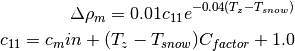
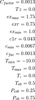
smrf.envphys.snow.marks2017(Tpp, pp)[source]¶ A new accumulated snow density model that accounts for compaction. The model builds upon
piecewise_susong1999()by adding effects from compaction. Of four mechanisms for compaction, this model accounts for compaction by destructive metmorphosism and overburden. These two processes are accounted for by calculating a proportionalility using data from Kojima, Yosida and Mellor. The overburden is in part estimated using total storm deposition, where storms are defined intracking_by_station(). Once this is determined the final snow density is applied through the entire storm only varying with hourly temperature.- Snow Density:

- Overburden Proportionality:

- Metmorphism Proportionality:
- Constants:
Parameters: - Tpp – Numpy array of a single hour of temperature, use dew point if available [degrees C].
- pp – Numpy array representing the total amount of precip deposited during a storm in millimeters
Returns: - rho_s (numpy.array) - Density of the fresh snow in kg/m^3.
- swe (numpy.array) - Snow water equivalent.
- pcs (numpy.array) - Percent of the precipitation that is
- snow in values 0.0-1.0.
- rho_ns (numpy.array) - Density of the uncompacted snow, which
- is equivalent to the output from
piecewise_susong1999().
- d_rho_c (numpy.array) - Prportional coefficient for
- compaction from overburden.
- d_rho_m (numpy.array) - Proportional coefficient for
- compaction from melt.
- rho_s (numpy.array) - Final density of the snow [kg/m^3].
- rho (numpy.array) - Density of the precipitation, which
- continuously ranges from low density snow to pure liquid water (50-1000 kg/m^3).
- zs (numpy.array) - Snow height added from the precipitation.
Return type: dictionary
-
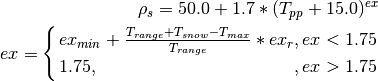
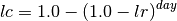
smrf.envphys.snow.piecewise_susong1999(Tpp, precip, Tmax=0.0, Tmin=-10.0, check_temps=True)[source]¶ Follows
susong1999()but is the piecewise form of table shown there. This model adds to the former by accounting for liquid water effect near 0.0 Degrees C.The table was estimated by Danny Marks in 2017 which resulted in the piecewise equations below:
- Percent Snow:
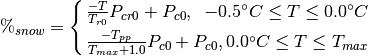
- Snow Density:
Parameters: - Tpp – A numpy array of temperature, use dew point temperature if available [degree C].
- precip – A numpy array of precip in millimeters.
- Tmax – Max temperature that snow density is modeled. Default is 0.0 Degrees C.
- Tmin – Minimum temperature that snow density is changing. Default is -10.0 Degrees C.
- check_temps – A boolean value check to apply special temperature constraints,
this is done using
check_temperature(). Default is True.
Returns: - pcs (numpy.array) - Percent of the precipitation that is snow
- in values 0.0-1.0.
- rho_s (numpy.array) - Density of the fresh snow in kg/m^3.
Return type: dictionary
-
smrf.envphys.snow.susong1999(temperature, precipitation)[source]¶ Follows the IPW command mkprecip
The precipitation phase, or the amount of precipitation falling as rain or snow, can significantly alter the energy and mass balance of the snowpack, either leading to snow accumulation or inducing melt [5] [6]. The precipitation phase and initial snow density are based on the precipitation temperature (the distributed dew point temperature) and are estimated after Susong et al (1999) [23]. The table below shows the relationship to precipitation temperature:
Min Temp Max Temp Percent snow Snow density [deg C] [deg C] [%] [kg/m^3] -Inf -5 100 75 -5 -3 100 100 -3 -1.5 100 150 -1.5 -0.5 100 175 -0.5 0 75 200 0 0.5 25 250 0.5 Inf 0 0 Parameters: - - numpy array of precipitation values [mm] (precipitation) –
- - array of temperature values, use dew point temperature (temperature) –
- available [degrees C] (if) –
Returns: Return type: dictionary
- perc_snow (numpy.array) - Percent of the precipitation that is snow
- in values 0.0-1.0.
- rho_s (numpy.array) - Snow density values in kg/m^3.
smrf.envphys.storms module
Created on March 14, 2017 Originally written by Scott Havens in 2015 @author: Micah Johnson
-
smrf.envphys.storms.clip_and_correct(precip, storms, stations=[])[source]¶ Meant to go along with the storm tracking, we correct the data here by adding in the precip we would miss by ignoring it. This is mostly because will get rain on snow events when there is snow because of the storm definitions and still try to distribute precip data.
Parameters: - precip – Vector station data representing the measured precipitation
- storms – Storm list with dictionaries as defined in
tracking_by_station() - stations – Desired stations that are being used for clipping. If stations is not passed, then use all in the dataframe
Returns: The correct precip that ensures there is no precip outside of the defined storms with the clipped amount of precip proportionally added back to storms.
Created May 3, 2017 @author: Micah Johnson
-
smrf.envphys.storms.storms(precipitation, perc_snow, mass=1, time=4, stormDays=None, stormPrecip=None, ps_thresh=0.5)[source]¶ Calculate the decimal days since the last storm given a precip time series, percent snow, mass threshold, and time threshold
- Will look for pixels where perc_snow > 50% as storm locations
- A new storm will start if the mass at the pixel has exceeded the mass
- limit, this ensures that the enough has accumulated
Parameters: - precipitation – Precipitation values
- perc_snow – Precent of precipitation that was snow
- mass – Threshold for the mass to start a new storm
- time – Threshold for the time to start a new storm
- stormDays – If specified, this is the output from a previous run of storms
- stormPrecip – Keeps track of the total storm precip
Returns: - stormDays - Array representing the days since the last storm at
- a pixel
- stormPrecip - Array representing the precip accumulated during
- the most recent storm
Return type: tuple
Created April 17, 2015 @author: Scott Havens
-
smrf.envphys.storms.time_since_storm(precipitation, perc_snow, time_step=0.041666666666666664, mass=1.0, time=4, stormDays=None, stormPrecip=None, ps_thresh=0.5)[source]¶ Calculate the decimal days since the last storm given a precip time series, percent snow, mass threshold, and time threshold
- Will look for pixels where perc_snow > 50% as storm locations
- A new storm will start if the mass at the pixel has exceeded the mass
- limit, this ensures that the enough has accumulated
Parameters: - precipitation – Precipitation values
- perc_snow – Percent of precipitation that was snow
- time_step – Step in days of the model run
- mass – Threshold for the mass to start a new storm
- time – Threshold for the time to start a new storm
- stormDays – If specified, this is the output from a previous run of storms else it will be set to the date_time value
- stormPrecip – Keeps track of the total storm precip
Returns: - stormDays - Array representing the days since the last storm at
- a pixel
- stormPrecip - Array representing the precip accumulated during
- the most recent storm
Return type: tuple
Created Janurary 5, 2016 @author: Scott Havens
-
smrf.envphys.storms.time_since_storm_basin(precipitation, storm, stormid, storming, time, time_step=0.041666666666666664, stormDays=None)[source]¶ Calculate the decimal days since the last storm given a precip time series, days since last storm in basin, and if it is currently storming
- Will assign uniform decimal days since last storm to every pixel
Parameters: - precipitation – Precipitation values
- storm – current or most recent storm
- time_step – step in days of the model run
- last_storm_day_basin – time since last storm for the basin
- stormid – ID of current storm
- storming – if it is currently storming
- time – current time
- stormDays – unifrom days since last storm on pixel basis
Returns: unifrom days since last storm on pixel basis
Return type: stormDays
Created May 9, 2017 @author: Scott Havens modified by Micah Sandusky
-
smrf.envphys.storms.time_since_storm_pixel(precipitation, dpt, perc_snow, storming, time_step=0.041666666666666664, stormDays=None, mass=1.0, ps_thresh=0.5)[source]¶ Calculate the decimal days since the last storm given a precip time series
- Will assign decimal days since last storm to every pixel
Parameters: - precipitation – Precipitation values
- dpt – dew point values
- perc_snow – percent_snow values
- storming – if it is stomring
- time_step – step in days of the model run
- stormDays – unifrom days since last storm on pixel basis
- mass – Threshold for the mass to start a new storm
- ps_thresh – Threshold for percent_snow
Returns: days since last storm on pixel basis
Return type: stormDays
Created October 16, 2017 @author: Micah Sandusky
-
smrf.envphys.storms.tracking_by_basin(precipitation, time, storm_lst, time_steps_since_precip, is_storming, mass_thresh=0.01, steps_thresh=2)[source]¶ Parameters: - precipitation – precipitation values
- time – Time step that smrf is on
- time_steps_since_precip – time steps since the last precipitation
- storm_lst –
list that store the storm cycles in order. A storm is recorded by its start and its end. The list is passed by reference and modified internally. Each storm entry should be in the format of: [{start:Storm Start, end:Storm End}]
- e.g.
- [
{start:date_time1,end:date_time2},
{start:date_time3,end:date_time4},
]
#would be a two storms
- mass_thresh – mass amount that constitutes a real precip event, default = 0.0.
- steps_thresh – Number of time steps that constitutes the end of a precip event, default = 2 steps (typically 2 hours)
Returns: storm_lst - updated storm_lst time_steps_since_precip - updated time_steps_since_precip is_storming - True or False whether the storm is ongoing or not
Return type: tuple
Created March 3, 2017 @author: Micah Johnson
-
smrf.envphys.storms.tracking_by_station(precip, mass_thresh=0.01, steps_thresh=3)[source]¶ Processes the vector station data prior to the data being distributed
Parameters: - precipitation – precipitation values
- time – Time step that smrf is on
- time_steps_since_precip – time steps since the last precipitation
- storm_lst –
list that store the storm cycles in order. A storm is recorded by its start and its end. The list is passed by reference and modified internally. Each storm entry should be in the format of: [{start:Storm Start, end:Storm End}]
- e.g.
- [
{start:date_time1,end:date_time2,’BOG1’:100, ‘ATL1’:85},
{start:date_time3,end:date_time4,’BOG1’:50, ‘ATL1’:45},
]
#would be a two storms at stations BOG1 and ATL1
- mass_thresh – mass amount that constitutes a real precip event, default = 0.01.
- steps_thresh – Number of time steps that constitutes the end of a precip event, default = 2 steps (typically 2 hours)
Returns: - storms - A list of dictionaries containing storm start,stop,
- mass accumulated, of given storm.
- storm_count - A total number of storms found
Return type: tuple
Created April 24, 2017 @author: Micah Johnson
smrf.envphys.radiation module
Created on Apr 17, 2015 @author: scott
-
smrf.envphys.radiation.albedo(telapsed, cosz, gsize, maxgsz, dirt=2)[source]¶ Calculate the abedo, adapted from IPW function albedo
Parameters: - - time since last snow storm (telapsed) –
- - cosine local solar illumination angle matrix (cosz) –
- - gsize is effective grain radius of snow after last storm (gsize) –
- - maxgsz is maximum grain radius expected from grain growth (maxgsz) – (mu m)
- - dirt is effective contamination for adjustment to visible (dirt) – albedo (usually between 1.5-3.0)
Returns: Returns a tuple containing the visible and IR spectral albedo
- alb_v (numpy.array) - albedo for visible specturm
- alb_ir (numpy.array) - albedo for ir spectrum
Return type: tuple
Created April 17, 2015 Modified July 23, 2015 - take image of cosz and calculate albedo for
one time stepScott Havens
-
smrf.envphys.radiation.cf_cloud(beam, diffuse, cf)[source]¶ Correct beam and diffuse irradiance for cloud attenuation at a single time, using input clear-sky global and diffuse radiation calculations supplied by locally modified toporad or locally modified stoporad
Parameters: - beam – global irradiance
- diffuse – diffuse irradiance
- cf – cloud attenuation factor - actual irradiance / clear-sky irradiance
Returns: cloud corrected gobal irradiance c_drad: cloud corrected diffuse irradiance
Return type: c_grad
20150610 Scott Havens - adapted from cloudcalc.c
-
smrf.envphys.radiation.decay_alb_hardy(litter, veg_type, storm_day, alb_v, alb_ir)[source]¶ Find a decrease in albedo due to litter acccumulation using method from [24] with storm_day as input.
Where
 is the fractional litter coverage and
  is the daily
litter rate of the forest. The new albedo is a weighted average of the calculated albedo
for the clean snow and the albedo of the litter.
is the daily
litter rate of the forest. The new albedo is a weighted average of the calculated albedo
for the clean snow and the albedo of the litter.Note: uses input of l_rate (litter rate) from config which is based on veg type. This is decimal percent litter coverage per day
Parameters: - litter – A dictionary of values for default,albedo,41,42,43 veg types
- veg_type – An image of the basin’s NLCD veg type
- storm_day – numpy array of decimal day since last storm
- alb_v – numpy array of albedo for visibile spectrum
- alb_ir – numpy array of albedo for IR spectrum
- alb_litter – albedo of pure litter
Returns: Returns a tuple containing the corrected albedo arrays based on date, veg type - alb_v (numpy.array) - albedo for visible specturm
- alb_ir (numpy.array) - albedo for ir spectrum
Return type: tuple
Created July 19, 2017 Micah Sandusky
-
smrf.envphys.radiation.decay_alb_power(veg, veg_type, start_decay, end_decay, t_curr, pwr, alb_v, alb_ir)[source]¶ Find a decrease in albedo due to litter acccumulation. Decay is based on max decay, decay power, and start and end dates. No litter decay occurs before start_date. Fore times between start and end of decay,
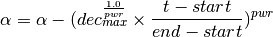
Where
 is albedo,
  is the maximum decay for albedo,
 is the decay power,
  ,
,  , and
, and  are the current,
start, and end times for the litter decay.
are the current,
start, and end times for the litter decay.Parameters: - start_decay – date to start albedo decay (datetime)
- end_decay – date at which to end albedo decay curve (datetime)
- t_curr – datetime object of current timestep
- pwr – power for power law decay
- alb_v – numpy array of albedo for visibile spectrum
- alb_ir – numpy array of albedo for IR spectrum
Returns: Returns a tuple containing the corrected albedo arrays based on date, veg type - alb_v (numpy.array) - albedo for visible specturm
- alb_ir (numpy.array) - albedo for ir spectrum
Return type: tuple
Created July 18, 2017 Micah Sandusky
-
smrf.envphys.radiation.get_hrrr_cloud(df_solar, df_meta, logger, lat, lon)[source]¶ Take the combined solar from HRRR and use the two stream calculation at the specific HRRR pixels to find the cloud_factor.
Parameters: - - solar dataframe from hrrr (df_solar) –
- - meta_data from hrrr (df_meta) –
- - smrf logger (logger) –
- - basin lat (lat) –
- - basin lon (lon) –
Returns: df_cf - cloud factor dataframe in same format as df_solar input
-
smrf.envphys.radiation.hor1f(x, z, offset=1)[source]¶ BROKEN: Haven’t quite figured this one out
Calculate the horizon pixel for all x,z This mimics the algorthim from Dozier 1981 and the hor1f.c from IPW
Works backwards from the end but looks forwards for the horizon
xrange stops one index before [stop]
Parameters: - - horizontal distances for points (x) –
- - elevations for the points (z) –
Returns: h - index to the horizon point
20150601 Scott Havens
-
smrf.envphys.radiation.hor1f_simple(z)[source]¶ Calculate the horizon pixel for all x,z This mimics the simple algorthim from Dozier 1981 to help understand how it’s working
Works backwards from the end but looks forwards for the horizon 90% faster than rad.horizon
Parameters: - - horizontal distances for points (x) –
- - elevations for the points (z) –
Returns: h - index to the horizon point
20150601 Scott Havens
-
smrf.envphys.radiation.hord(z)[source]¶ Calculate the horizon pixel for all x,z This mimics the simple algorthim from Dozier 1981 to help understand how it’s working
Works backwards from the end but looks forwards for the horizon 90% faster than rad.horizon
- Args::
- x - horizontal distances for points z - elevations for the points
Returns: h - index to the horizon point 20150601 Scott Havens
-
smrf.envphys.radiation.ihorizon(x, y, Z, azm, mu=0, offset=2, ncores=0)[source]¶ Calculate the horizon values for an entire DEM image for the desired azimuth
Assumes that the step size is constant
Parameters: - - vector of x-coordinates (X) –
- - vector of y-coordinates (Y) –
- - matrix of elevation data (Z) –
- - azimuth to calculate the horizon at (azm) –
- - 0 -> calculate cos (mu) –
- >0 -> calculate a mask whether or not the point can see the sun
Returns: - H - if mask=0 cosine of the local horizonal angles
- if mask=1 index along line to the point
20150602 Scott Havens
-
smrf.envphys.radiation.model_solar(dt, lat, lon, tau=0.2, tzone=0)[source]¶ Model solar radiation at a point Combines sun angle, solar and two stream
Parameters: - - datetime object (dt) –
- - latitude (lat) –
- - longitude (lon) –
- - optical depth (tau) –
- - time zone (tzone) –
Returns: corrected solar radiation
-
smrf.envphys.radiation.shade(slope, aspect, azimuth, cosz=None, zenith=None)[source]¶ Calculate the cosize of the local illumination angle over a DEM
Solves the following equation cos(ts) = cos(t0) * cos(S) + sin(t0) * sin(S) * cos(phi0 - A)
- where
- t0 is the illumination angle on a horizontal surface phi0 is the azimuth of illumination S is slope in radians A is aspect in radians
Slope and aspect are expected to come from the IPW gradient command. Slope is stored as sin(S) with range from 0 to 1. Aspect is stored as radians from south (aspect 0 is toward the south) with range from -pi to pi, with negative values to the west and positive values to the east
Parameters: - slope – numpy array of sine of slope angles
- aspect – numpy array of aspect in radians from south
- azimuth – azimuth in degrees to the sun -180..180 (comes from sunang)
- cosz – cosize of the zeinith angle 0..1 (comes from sunang)
- zenith – the solar zenith angle 0..90 degrees
At least on of the cosz or zenith must be specified. If both are specified the zenith is ignored
Returns: numpy matrix of the cosize of the local illumination angle cos(ts) Return type: mu The python shade() function is an interpretation of the IPW shade() function and follows as close as possible. All equations are based on Dozier & Frew, 1990. ‘Rapid calculation of Terrain Parameters For Radiation Modeling From Digitial Elevation Data,’ IEEE TGARS
20150106 Scott Havens
-
smrf.envphys.radiation.shade_thread(queue, date, slope, aspect, zenith=None)[source]¶ See shade for input argument descriptions
Parameters: - queue – queue with illum_ang, cosz, azimuth
- date_time – loop through dates to accesss queue
20160325 Scott Havens
-
smrf.envphys.radiation.solar_ipw(d, w=[0.28, 2.8])[source]¶ Wrapper for the IPW solar function
Solar calculates exoatmospheric direct solar irradiance. If two arguments to -w are given, the integral of solar irradiance over the range will be calculated. If one argument is given, the spectral irradiance will be calculated.
If no wavelengths are specified on the command line, single wavelengths in um will be read from the standard input and the spectral irradiance calculated for each.
Parameters: - - [um um2] If two arguments are given, the integral of solar (w) – irradiance in the range um to um2 will be calculated. If one argument is given, the spectral irradiance will be calculated.
- - date object, This is used to calculate the solar radius vector (d) – which divides the result
Returns: s - direct solar irradiance
20151002 Scott Havens
-
smrf.envphys.radiation.sunang(date, lat, lon, zone=0, slope=0, aspect=0)[source]¶ Wrapper for the IPW sunang function
Parameters: - - date to calculate sun angle for (date) –
- - latitude in decimal degrees (lat) –
- - longitude in decimal degrees (lon) –
- - The time values are in the time zone which is min minutes (zone) – west of Greenwich (default: 0). For example, if input times are in Pacific Standard Time, then min would be 480.
- slope (default=0) –
- aspect (default=0) –
Returns: cosz - cosine of the zeinith angle azimuth - solar azimuth
Created April 17, 2015 Scott Havnes
-
smrf.envphys.radiation.sunang_thread(queue, date, lat, lon, zone=0, slope=0, aspect=0)[source]¶ See sunang for input descriptions
Parameters: - queue – queue with cosz, azimuth
- date – loop through dates to accesss queue, must be same as rest of queues
20160325 Scott Havens
-
smrf.envphys.radiation.twostream(mu0, S0, tau=0.2, omega=0.85, g=0.3, R0=0.5, d=False)[source]¶ Wrapper for the twostream.c IPW function
Provides twostream solution for single-layer atmosphere over horizontal surface, using solution method in: Two-stream approximations to radiative transfer in planetary atmospheres: a unified description of existing methods and a new improvement, Meador & Weaver, 1980, or will use the delta-Eddington method, if the -d flag is set (see: Wiscombe & Joseph 1977).
Parameters: - - The cosine of the incidence angle is cos (mu0) –
- - Do not force an error if mu0 is <= 0.0; set all outputs to 0.0 and (0) – go on. Program will fail if incidence angle is <= 0.0, unless -0 has been set.
- - The optical depth is tau. 0 implies an infinite optical depth. (tau) –
- - The single-scattering albedo is omega. (omega) –
- - The asymmetry factor is g. (g) –
- - The reflectance of the substrate is R0. If R0 is negative, it (R0) – will be set to zero.
- - The direct beam irradiance is S0 This is usually the solar (S0) – constant for the specified wavelength band, on the specified date, at the top of the atmosphere, from program solar. If S0 is negative, it will be set to 1/cos, or 1 if cos is not specified.
- - The delta-Eddington method will be used. (d) –
Returns: R[0] - reflectance R[1] - transmittance R[2] - direct transmittance R[3] - upwelling irradiance R[4] - total irradiance at bottom R[5] - direct irradiance normal to beam
20151002 Scott Havens
smrf.envphys.thermal_radiation module
The module contains various physics calculations needed for estimating the thermal radition and associated values.
-
smrf.envphys.thermal_radiation.Angstrom1918(ta, ea)[source]¶ Estimate clear-sky downwelling long wave radiation from Angstrom (1918) [15] as cited by Niemela et al (2001) [16] using the equation:

Where
 is the vapor pressure.
Parameters: - ta – distributed air temperature [degree C]
- ea – distrubted vapor pressure [kPa]
Returns: clear sky long wave radiation [W/m2]
20170509 Scott Havens
-
smrf.envphys.thermal_radiation.Crawford1999(th, ta, cloud_factor)[source]¶ Cloud correction is based on Crawford and Duchon (1999) [20]

where
 is the ratio of measured solar radiation to the
clear sky irradiance.
is the ratio of measured solar radiation to the
clear sky irradiance.Parameters: - th – clear sky thermal radiation [W/m2]
- ta – temperature in Celcius that the clear sky thermal radiation was calcualted from [C]
- cloud_factor – fraction of sky that are not clouds, 1 equals no clouds, 0 equals all clouds
Returns: cloud corrected clear sky thermal radiation
20170515 Scott Havens
-
smrf.envphys.thermal_radiation.Dilly1998(ta, ea)[source]¶ Estimate clear-sky downwelling long wave radiation from Dilley & O’Brian (1998) [13] using the equation:
Where
 is the air temperature and
  is the amount of
precipitable water. The preipitable water is estimated as
is the amount of
precipitable water. The preipitable water is estimated as
 from Prata (1996) [14].
Parameters: - ta – distributed air temperature [degree C]
- ea – distrubted vapor pressure [kPa]
Returns: clear sky long wave radiation [W/m2]
20170509 Scott Havens
-
smrf.envphys.thermal_radiation.Garen2005(th, cloud_factor)[source]¶ Cloud correction is based on the relationship in Garen and Marks (2005) [17] between the cloud factor and measured long wave radiation using measurement stations in the Boise River Basin.

Parameters: - th – clear sky thermal radiation [W/m2]
- cloud_factor – fraction of sky that are not clouds, 1 equals no clouds, 0 equals all clouds
Returns: cloud corrected clear sky thermal radiation
20170515 Scott Havens
-
smrf.envphys.thermal_radiation.Kimball1982(th, ta, ea, cloud_factor)[source]¶ Cloud correction is based on Kimball et al. (1982) [19]
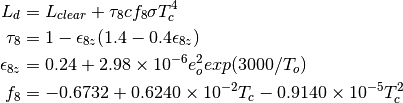
where the original Kimball et al. (1982) [19] was for multiple cloud layers, which was simplified to one layer.
 is
the cloud temperature and is assumed to be 11 K cooler than .
is
the cloud temperature and is assumed to be 11 K cooler than .Parameters: - th – clear sky thermal radiation [W/m2]
- ta – temperature in Celcius that the clear sky thermal radiation was calcualted from [C]
- ea – distrubted vapor pressure [kPa]
- cloud_factor – fraction of sky that are not clouds, 1 equals no clouds, 0 equals all clouds
Returns: cloud corrected clear sky thermal radiation
20170515 Scott Havens
-
smrf.envphys.thermal_radiation.Prata1996(ta, ea)[source]¶ Estimate clear-sky downwelling long wave radiation from Prata (1996) [14] using the equation:

Where
is the amount of precipitable water. The preipitable
water is estimated as from Prata (1996)
[14].Parameters: - ta – distributed air temperature [degree C]
- ea – distrubted vapor pressure [kPa]
Returns: clear sky long wave radiation [W/m2]
20170509 Scott Havens
-
smrf.envphys.thermal_radiation.Unsworth1975(th, ta, cloud_factor)[source]¶ Cloud correction is based on Unsworth and Monteith (1975) [18]

where

Parameters: - th – clear sky thermal radiation [W/m2]
- ta – temperature in Celcius that the clear sky thermal radiation was calcualted from [C] cloud_factor: fraction of sky that are not clouds, 1 equals no clouds, 0 equals all clouds
Returns: cloud corrected clear sky thermal radiation
20170515 Scott Havens
-
smrf.envphys.thermal_radiation.brutsaert(ta, l, ea, z, pa)[source]¶ Calculate atmosphere emissivity from Brutsaert (1975):cite:Brutsaert:1975
Parameters: - ta – air temp (K)
- l – temperature lapse rate (deg/m)
- ea – vapor pressure (Pa)
- z – elevation (z)
- pa – air pressure (Pa)
Returns: atmosphericy emissivity
20151027 Scott Havens
-
smrf.envphys.thermal_radiation.calc_long_wave(e, ta)[source]¶ Apply the Stephan-Boltzman equation for longwave
-
smrf.envphys.thermal_radiation.hysat(pb, tb, L, h, g, m)[source]¶ integral of hydrostatic equation over layer with linear temperature variation
Parameters: - pb – base level pressure
- tb – base level temp [K]
- L – lapse rate [deg/km]
- h – layer thickness [km]
- g – grav accel [m/s^2]
- m – molec wt [kg/kmole]
Returns: hydrostatic results
20151027 Scott Havens
-
smrf.envphys.thermal_radiation.precipitable_water(ta, ea)[source]¶ Estimate the precipitable water from Prata (1996) [14]
-
smrf.envphys.thermal_radiation.sati(tk)[source]¶ saturation vapor pressure over ice. From IPW sati
Parameters: tk – temperature in Kelvin Returns: saturated vapor pressure over ice 20151027 Scott Havens
-
smrf.envphys.thermal_radiation.satw(tk)[source]¶ Saturation vapor pressure of water. from IPW satw
Parameters: tk – temperature in Kelvin Returns: saturated vapor pressure over water 20151027 Scott Havens
-
smrf.envphys.thermal_radiation.thermal_correct_canopy(th, ta, tau, veg_height, height_thresh=2)[source]¶ Correct thermal radiation for vegitation. It will only correct for pixels where the veg height is above a threshold. This ensures that the open areas don’t get this applied. Vegitation temp is assumed to be at air temperature
Parameters: - th – thermal radiation
- ta – air temperature [C]
- tau – transmissivity of the canopy
- veg_height – vegitation height for each pixel
- height_thresh – threshold hold for height to say that there is veg in the pixel
Returns: corrected thermal radiation
Equations from Link and Marks 1999 [10]
20150611 Scott Havens
-
smrf.envphys.thermal_radiation.thermal_correct_terrain(th, ta, viewf)[source]¶ Correct the thermal radiation for terrain assuming that the terrain is at the air temperature and the pixel and a sky view
Parameters: - th – thermal radiation
- ta – air temperature [C]
- viewf – sky view factor from view_f
Returns: corrected thermal radiation
20150611 Scott Havens
-
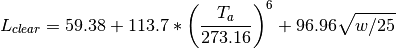
smrf.envphys.thermal_radiation.topotherm(ta, tw, z, skvfac)[source]¶ Calculate the clear sky thermal radiation. topotherm calculates thermal radiation from the atmosphere corrected for topographic effects, from near surface air temperature Ta, dew point temperature DPT, and elevation. Based on a model by Marks and Dozier (1979) :citeL`Marks&Dozier:1979`.
Parameters: - ta – air temperature [C]
- tw – dew point temperature [C]
- z – elevation [m]
- skvfac – sky view factor
Returns: Long wave (thermal) radiation corrected for terrain
20151027 Scott Havens