smrf.distribute package¶

A base distribution method smrf.distribute.image_data is used in SMRF to ensure that all variables are distributed in the same manner. The additional benefit is that when new methods are added to smrf.spatial, the new method will only need to be added into smrf.distribute.image_data and will be immediately available to all other distribution variables.

smrf.distribute.image_data module¶

class smrf.distribute.image_data.image_data(variable)[source]¶

Bases: object

A base distribution method in SMRF that will ensure all variables are distributed in the same manner. Other classes will be initialized using this base class.

class ta(smrf.distribute.image_data):
    '''
    This is the ta class extending the image_data base class
    '''

Parameters:	variable (str) – Variable name for the class
Returns:	A `smrf.distribute.image_data` class instance

variable¶: The name of the variable that this class will become

[variable_name]: The variable will have the distributed data

[other_attribute]: The distributed data can also be stored as another attribute specified in _distribute

config¶: Parsed dictionary from the configuration file for the variable

stations¶: The stations to be used for the variable, if set, in alphabetical order

metadata¶: The metadata Pandas dataframe containing the station information from smrf.data.loadData or smrf.data.loadGrid

idw¶: Inverse distance weighting instance from smrf.spatial.idw.IDW

dk¶: Detrended kriging instance from smrf.spatial.dk.dk.DK

grid¶: Gridded interpolation instance from smrf.spatial.grid.GRID

_distribute(data, other_attribute=None, zeros=None)[source]¶

Distribute the data using the defined distribution method in config

Parameters:	data – Pandas dataframe for a single time step other_attribute (str) – By default, the distributed data matrix goes into self.variable but this specifies another attribute in self zeros – data values that should be treated as zeros (not used)
Raises:	`Exception` – If all input data is NaN

_initialize(topo, metadata)[source]¶

Initialize the distribution based on the parameters in config.

Parameters:	topo – `smrf.data.loadTopo.topo` instance contain topographic data and infomation metadata – metadata Pandas dataframe containing the station metadata from `smrf.data.loadData` or `smrf.data.loadGrid`
Raises:	`Exception` – If the distribution method could not be determined, must be idw, dk, or grid

To do:

make a single call to the distribution initialization
each dist (idw, dk, grid) takes the same inputs and returns the

same

getConfig(cfg)[source]¶

Check the configuration that was set by the user for the variable that extended this class. Checks for standard distribution parameters that are common across all variables and assigns to the class instance. Sets the config and stations attributes.

Parameters:	cfg (dict) – dict from the [variable]

getStations(config)[source]¶

Determines the stations from the [variable] section of the configuration file.

Parameters:	config (dict) – dict from the [variable]

post_processor(output_func)[source]¶

Each distributed variable has the oppurtunity to do post processing on a sub variable. This is necessary in cases where the post proecessing might need to be done on a different timescale than that of the main loop.

Should be redefined in the individual variable module.

smrf.distribute.air_temp module¶

class smrf.distribute.air_temp.ta(taConfig)[source]¶

Bases: smrf.distribute.image_data.image_data

The ta class allows for variable specific distributions that go beyond the base class.

Air temperature is a relatively simple variable to distribute as it does not rely on any other variables, but has many variables that depend on it. Air temperature typically has a negative trend with elevation and performs best when detrended. However, even with a negative trend, it is possible to have instances where the trend does not apply, for example a temperature inversion or cold air pooling. These types of conditions will have unintended concequences on variables that use the distributed air temperature.

Parameters:	taConfig – The [air_temp] section of the configuration file

config¶: configuration from [air_temp] section

air_temp¶: numpy array of the air temperature

stations¶: stations to be used in alphabetical order

output_variables¶: Dictionary of the variables held within class smrf.distribute.air_temp.ta that specifies the units and long_name for creating the NetCDF output file.

variable¶: ‘air_temp’

distribute(data)[source]¶

Distribute air temperature given a Panda’s dataframe for a single time step. Calls smrf.distribute.image_data.image_data._distribute.

Parameters:	data – Pandas dataframe for a single time step from air_temp

distribute_thread(queue, data)[source]¶

Distribute the data using threading and queue. All data is provided and distribute_thread will go through each time step and call smrf.distribute.air_temp.ta.distribute then puts the distributed data into queue['air_temp'].

Parameters:	queue – queue dictionary for all variables data – pandas dataframe for all data, indexed by date time

initialize(topo, data)[source]¶

Initialize the distribution, soley calls smrf.distribute.image_data.image_data._initialize.

Parameters:	topo – `smrf.data.loadTopo.topo` instance contain topographic data and infomation metadata – metadata Pandas dataframe containing the station metadata from `smrf.data.loadData` or `smrf.data.loadGrid`

smrf.distribute.albedo module¶

class smrf.distribute.albedo.albedo(albedoConfig)[source]¶

Bases: smrf.distribute.image_data.image_data

The albedo class allows for variable specific distributions that go beyond the base class.

The visible (280-700nm) and infrared (700-2800nm) albedo follows the relationships described in Marks et al. (1992) [4]. The albedo is a function of the time since last storm, the solar zenith angle, and grain size. The time since last storm is tracked on a pixel by pixel basis and is based on where there is significant accumulated distributed precipitation. This allows for storms to only affect a small part of the basin and have the albedo decay at different rates for each pixel.

Parameters:	albedoConfig – The [albedo] section of the configuration file

albedo_vis¶: numpy array of the visible albedo

albedo_ir¶: numpy array of the infrared albedo

config¶: configuration from [albedo] section

min¶: minimum value of albedo is 0

max¶: maximum value of albedo is 1

stations¶: stations to be used in alphabetical order

output_variables¶: Dictionary of the variables held within class smrf.distribute.albedo.albedo that specifies the units and long_name for creating the NetCDF output file.

variable¶: ‘albedo’

distribute(current_time_step, cosz, storm_day)[source]¶

Distribute air temperature given a Panda’s dataframe for a single time step. Calls smrf.distribute.image_data.image_data._distribute.

Parameters:	current_time_step – Current time step in datetime object cosz – numpy array of the illumination angle for the current time step storm_day – numpy array of the decimal days since it last snowed at a grid cell

distribute_thread(queue, date)[source]¶

Distribute the data using threading and queue

Parameters:	queue – queue dict for all variables date – dates to loop over

Output:

Changes the queue albedo_vis, albedo_ir: for the given date

initialize(topo, data)[source]¶

Initialize the distribution, calls image_data.image_data._initialize()

Parameters:	topo – smrf.data.loadTopo.topo instance contain topo data/info data – data dataframe containing the station data

smrf.distribute.precipitation module¶

class smrf.distribute.precipitation.ppt(pptConfig, start_date, time_step=60)[source]¶

Bases: smrf.distribute.image_data.image_data

The ppt class allows for variable specific distributions that go beyond the base class.

The instantaneous precipitation typically has a positive trend with elevation due to orographic effects. However, the precipitation distribution can be further complicated for storms that have isolated impact at only a few measurement locations, for example thunderstorms or small precipitation events. Some distirubtion methods may be better suited than others for capturing the trend of these small events with multiple stations that record no precipitation may have a negative impact on the distribution.

The precipitation phase, or the amount of precipitation falling as rain or snow, can significantly alter the energy and mass balance of the snowpack, either leading to snow accumulation or inducing melt [5] [6]. The precipitation phase and initial snow density estimated using a variety of models that can be set in the configuration file.

For more information on the available models, checkout snow.

After the precipitation phase is calculated, the storm infromation can be determined. The spatial resolution for which storm definitions are applied is based on the snow model thats selected.

The time since last storm is based on an accumulated precipitation mass threshold, the time elapsed since it last snowed, and the precipitation phase. These factors determine the start and end time of a storm that has produced enough precipitation as snow to change the surface albedo.

Parameters:	pptConfig – The [precip] section of the configuration file time_step – The time step in minutes of the data, defaults to 60

config¶: configuration from [precip] section

precip¶: numpy array of the precipitation

percent_snow¶: numpy array of the percent of time step that was snow

snow_density¶: numpy array of the snow density

storm_days¶: numpy array of the days since last storm

storm_total¶: numpy array of the precipitation mass for the storm

last_storm_day¶: numpy array of the day of the last storm (decimal day)

last_storm_day_basin¶: maximum value of last_storm day within the mask if specified

min¶: minimum value of precipitation is 0

max¶: maximum value of precipitation is infinite

stations¶: stations to be used in alphabetical order

output_variables¶: Dictionary of the variables held within class smrf.distribute.precipitation.ppt that specifies the units and long_name for creating the NetCDF output file.

variable¶: ‘precip’

distribute(data, dpt, precip_temp, ta, time, wind, temp, az, dir_round_cell, wind_speed, cell_maxus, mask=None)[source]¶

Distribute given a Panda’s dataframe for a single time step. Calls smrf.distribute.image_data.image_data._distribute.

The following steps are taken when distributing precip, if there is precipitation measured:

Distribute the instaneous precipitation from the measurement data
Determine the distributed precipitation phase based on the

precipitation temperature
Calculate the storms based on the accumulated mass, time since last

storm, and precipitation phase threshold

Parameters:

data – Pandas dataframe for a single time step from precip
dpt – dew point numpy array that will be used for
precip_temp – numpy array of the precipitaiton temperature
ta – air temp numpy array
time – pass in the time were are currently on
wind – station wind speed at time step
temp – station air temperature at time step
az – numpy array for simulated wind direction
dir_round_cell – numpy array for wind direction in descriete incriments for referencing maxus at a specific direction
wind_speed – numpy array of wind speed
cell_maxus – numpy array for maxus at correct wind directions
mask – basin mask to apply to the storm days for calculating the last storm day for the basin

distribute_for_marks2017(data, precip_temp, ta, time, mask=None)[source]¶: Specialized distribute function for working with the new accumulated snow density model Marks2017 requires storm total and a corrected precipitation as to avoid precip between storms.

distribute_for_susong1999(data, ppt_temp, time, mask=None)[source]¶: Docs for susong1999

distribute_thread(queue, data, date, mask=None)[source]¶

Distribute the data using threading and queue. All data is provided and distribute_thread will go through each time step and call smrf.distribute.precip.ppt.distribute then puts the distributed data into the queue for:

percent_snow
snow_density
storm_days
last_storm_day_basin

Parameters:	queue – queue dictionary for all variables data – pandas dataframe for all data, indexed by date time

smrf.distribute.soil_temp module¶

class smrf.distribute.soil_temp.ts(soilConfig, tempDir=None)[source]¶

Bases: smrf.distribute.image_data.image_data

The ts class allows for variable specific distributions that go beyond the base class.

Soil temperature is simply set to a constant value during initialization. If soil temperature measurements are available, the values can be distributed using the distribution methods.

Parameters:	soilConfig – The [soil] section of the configuration file tempDir – location of temp/working directory (default=None)

config¶: configuration from [soil] section

soil_temp¶: numpy array of the soil temperature

stations¶: stations to be used in alphabetical order

output_variables¶: Dictionary of the variables held within class smrf.distribute.soil_temp.ts that specifies the units and long_name for creating the NetCDF output file.

variable¶: ‘soil_temp’

distribute()[source]¶

No distribution is performed on soil temperature at the moment, method simply passes.

Parameters:	None –

initialize(topo, data)[source]¶

Initialize the distribution and set the soil temperature to a constant value based on the configuration file.

Parameters:	topo – `smrf.data.loadTopo.topo` instance contain topographic data and infomation metadata – data Pandas dataframe containing the station data, from `smrf.data.loadData` or `smrf.data.loadGrid`

smrf.distribute.solar module¶

class smrf.distribute.solar.solar(solarConfig, albedoConfig, stoporad_in, tempDir=None)[source]¶

Bases: smrf.distribute.image_data.image_data

The solar class allows for variable specific distributions that go beyond the base class.

Multiple steps are required to estimate solar radiation:

Terrain corrected clear sky radiation
Distribute a cloud factor and adjust modeled clear sky
Adjust solar radiation for vegetation effects
Calculate net radiation using the albedo

The Image Processing Workbench (IPW) includes a utility stoporad to model terrain corrected clear sky radiation over the DEM. Within stoporad, the radiation transfer model twostream simulates the clear sky radiation on a flat surface for a range of wavelengths through the atmosphere [7] [8] [9]. Terrain correction using the DEM adjusts for terrain shading and splits the clear sky radiation into beam and diffuse radiation.

The second step requires sites measuring solar radiation. The measured solar radiation is compared to the modeled clear sky radiation from twostream. The cloud factor is then the measured incoming solar radiation divided by the modeled radiation. The cloud factor can be computed on an hourly timescale if the measurement locations are of high quality. For stations that are less reliable, we recommend calculating a daily cloud factor which divides the daily integrated measured radiation by the daily integrated modeled radiation. This helps to reduce the problems that may be encountered from instrument shading, instrument calibration, or a time shift in the data. The calculated cloud factor at each station can then be distrubted using any of the method available in smrf.spatial. Since the cloud factor is not explicitly controlled by elevation like other variables, the values may be distributed without detrending to elevation. The modeled clear sky radiation (both beam and diffuse) are adjusted for clouds using smrf.envphys.radiation.cf_cloud.

The third step adjusts the cloud corrected solar radiation for vegetation affects, following the methods developed by Link and Marks (1999) [10]. The direct beam radiation is corrected by:

$R_b = S_b * exp( -\mu h / cos \theta )$

where $S_b$ is the above canopy direct radiation, $\mu$ is the extinction coefficient ( $m^{-1}$ ), $h$ is the canopy height ( $m$ ), $\theta$ is the solar zenith angle, and $R_b$ is the canopy adjusted direct radiation. Adjusting the diffuse radiation is performed by:

$R_d = \tau * R_d$

where $R_d$ is the diffuse adjusted radiation, $\tau$ is the optical transmissivity of the canopy, and $R_d$ is the above canopy diffuse radiation. Values for $\mu$ and $\tau$ can be found in Link and Marks (1999) [10], measured at study sites in Saskatchewan and Manitoba.

The final step for calculating the net solar radiation requires the surface albedo from smrf.distribute.albedo. The net radiation is the sum of the of beam and diffuse canopy adjusted radiation multipled by one minus the albedo.

Parameters:	solarConfig – configuration from [solar] section albedoConfig – configuration from [albedo] section stoporad_in – file path to the stoporad_in file created from `smrf.data.loadTopo.topo` tempDir – location of temp/working directory (default=None, which is the ‘WORKDIR’ environment variable)

config¶: configuration from [solar] section

albedoConfig¶: configuration from [albedo] section

stoporad_in¶: file path to the stoporad_in file created from smrf.data.loadTopo.topo

clear_ir_beam¶: numpy array modeled clear sky infrared beam radiation

clear_ir_diffuse¶: numpy array modeled clear sky infrared diffuse radiation

clear_vis_beam¶: numpy array modeled clear sky visible beam radiation

clear_vis_diffuse¶: numpy array modeled clear sky visible diffuse radiation

cloud_factor¶: numpy array distributed cloud factor

cloud_ir_beam¶: numpy array cloud adjusted infrared beam radiation

cloud_ir_diffuse¶: numpy array cloud adjusted infrared diffuse radiation

cloud_vis_beam¶: numpy array cloud adjusted visible beam radiation

cloud_vis_diffuse¶: numpy array cloud adjusted visible diffuse radiation

ir_file¶: temporary file from stoporad for infrared clear sky radiation

metadata¶: metadata for the station data

net_solar¶: numpy array for the calculated net solar radiation

output_variables¶: Dictionary of the variables held within class smrf.distribute.air_temp.ta that specifies the units and long_name for creating the NetCDF output file.

stations¶: stations to be used in alphabetical order

stoporad_in: file path to the stoporad_in file created from smrf.data.loadTopo.topo

tempDir¶: temporary directory for stoporad, will default to the WORKDIR environment variable

variable¶: solar

veg_height¶: numpy array of vegetation heights from smrf.data.loadTopo.topo

veg_ir_beam¶: numpy array vegetation adjusted infrared beam radiation

veg_ir_diffuse¶: numpy array vegetation adjusted infrared diffuse radiation

veg_k¶: numpy array of vegetation extinction coefficient from smrf.data.loadTopo.topo

veg_tau¶: numpy array of vegetation optical transmissivity from smrf.data.loadTopo.topo

veg_vis_beam¶: numpy array vegetation adjusted visible beam radiation

veg_vis_diffuse¶: numpy array vegetation adjusted visible diffuse radiation

vis_file¶: temporary file from stoporad for visible clear sky radiation

calc_ir(min_storm_day, wy_day, tz_min_west, wyear, cosz, azimuth)[source]¶

Run stoporad for the infrared bands

Parameters:

min_storm_day – decimal day of last storm for the entire basin, from smrf.distribute.precip.ppt.last_storm_day_basin
wy_day – day of water year, from radiation_dates
tz_min_west – time zone in minutes west from UTC, from radiation_dates
wyear – water year, from radiation_dates
cosz – cosine of the zenith angle for the basin, from smrf.envphys.radiation.sunang
azimuth – azimuth to the sun for the basin, from smrf.envphys.radiation.sunang

calc_net(albedo_vis, albedo_ir)[source]¶

Calculate the net radiation using the vegetation adjusted radiation. Sets net_solar.

Parameters:	albedo_vis – numpy array for visible albedo, from `smrf.distribute.albedo.albedo.albedo_vis` albedo_ir – numpy array for infrared albedo, from `smrf.distribute.albedo.albedo.albedo_ir`

calc_vis(min_storm_day, wy_day, tz_min_west, wyear, cosz, azimuth)[source]¶

Run stoporad for the visible bands

Parameters:

min_storm_day – decimal day of last storm for the entire basin, from smrf.distribute.precip.ppt.last_storm_day_basin
wy_day – day of water year, from radiation_dates
tz_min_west – time zone in minutes west from UTC, from radiation_dates
wyear – water year, from radiation_dates
cosz – cosine of the zenith angle for the basin, from smrf.envphys.radiation.sunang
azimuth – azimuth to the sun for the basin, from smrf.envphys.radiation.sunang

cloud_correct()[source]¶: Correct the modeled clear sky radiation for cloud cover using smrf.envphys.radiation.cf_cloud. Sets cloud_vis_beam and cloud_vis_diffuse.

distribute(data, illum_ang, cosz, azimuth, min_storm_day, albedo_vis, albedo_ir)[source]¶

Distribute air temperature given a Panda’s dataframe for a single time step. Calls smrf.distribute.image_data.image_data._distribute.

If the sun is up, i.e. cosz > 0, then the following steps are performed:

Distribute cloud factor
Model clear sky radiation
Cloud correct with smrf.distribute.solar.solar.cloud_correct
vegetation correct with

smrf.distribute.solar.solar.veg_correct
Calculate net radiation with

smrf.distribute.solar.solar.calc_net

If sun is down, then all calculated values will be set to None, signaling the output functions to put zeros in their place.

Parameters:

data – Pandas dataframe for a single time step from cloud_factor
cosz – cosine of the zenith angle for the basin, from smrf.envphys.radiation.sunang
azimuth – azimuth to the sun for the basin, from smrf.envphys.radiation.sunang
min_storm_day – decimal day of last storm for the entire basin, from smrf.distribute.precip.ppt.last_storm_day_basin
albedo_vis – numpy array for visible albedo, from smrf.distribute.albedo.albedo.albedo_vis
albedo_ir – numpy array for infrared albedo, from smrf.distribute.albedo.albedo.albedo_ir

distribute_thread(queue, data)[source]¶

Distribute the data using threading and queue. All data is provided and distribute_thread will go through each time step following the methods outlined in smrf.distribute.solar.solar.distribute. The data queues puts the distributed data into:

net_solar
cloud_factor

Parameters:	queue – queue dictionary for all variables data – pandas dataframe for all data, indexed by date time

distribute_thread_clear(queue, data, calc_type)[source]¶

Distribute the data using threading and queue. All data is provided and distribute_thread will go through each time step and model clear sky radiation with stoporad. The data queues puts the distributed data into:

clear_vis_beam
clear_vis_diffuse
clear_ir_beam
clear_ir_diffuse

initialize(topo, data)[source]¶

Initialize the distribution, soley calls smrf.distribute.image_data.image_data._initialize. Sets the following attributes:

veg_height
veg_tau
veg_k

Parameters:	topo – `smrf.data.loadTopo.topo` instance contain topographic data and infomation data – data Pandas dataframe containing the station data, from `smrf.data.loadData` or `smrf.data.loadGrid`

radiation_dates(date_time)[source]¶

Calculate some times based on the date for stoporad

Parameters:	date_time – date time object
Returns:	tuple containing: wy_day - day of water year from October 1 wyear - water year tz_min_west - minutes west of UTC for timezone
Return type:	(tuple)

veg_correct(illum_ang)[source]¶

Correct the cloud adjusted radiation for vegetation using smrf.envphys.radiation.veg_beam and smrf.envphys.radiation.veg_diffuse. Sets veg_vis_beam, veg_vis_diffuse, veg_ir_beam, and veg_ir_diffuse.

Parameters:	illum_ang – numpy array of the illumination angle over the DEM, from `smrf.envphys.radiation.sunang`

smrf.distribute.thermal module¶

class smrf.distribute.thermal.th(thermalConfig)[source]¶

Bases: smrf.distribute.image_data.image_data

The th class allows for variable specific distributions that go beyond the base class.

Thermal radiation, or long-wave radiation, is calculated based on the clear sky radiation emitted by the atmosphere. Multiple methods for calculating thermal radition exist and SMRF has 4 options for estimating clear sky thermal radiation. Selecting one of the options below will change the equations used. The methods were chosen based on the study by Flerchinger et al (2009) [11] who performed a model comparison using 21 AmeriFlux sites from North America and China.

Marks1979: The methods follow those developed by Marks and Dozier (1979) [12] that calculates the effective clear sky atmospheric emissivity using the distributed air temperature, distributed dew point temperature, and the elevation. The clear sky radiation is further adjusted for topographic affects based on the percent of the sky visible at any given point.
Dilley1998: $L_{clear} = 59.38 + 113.7 * \left( \frac{T_a}{273.16} \right)^6 + 96.96 \sqrt{w/25}$

References: Dilley and O’Brian (1998) [13]
Prata1996: $\epsilon_{clear} = 1 - (1 + w) * exp(-1.2 + 3w)^{1/2}$

References: Prata (1996) [14]
Angstrom1918: $\epsilon_{clear} = 0.83 - 0.18 * 10^{-0.067 e_a}$

References: Angstrom (1918) [15] as cityed by Niemela et al (2001) [16]

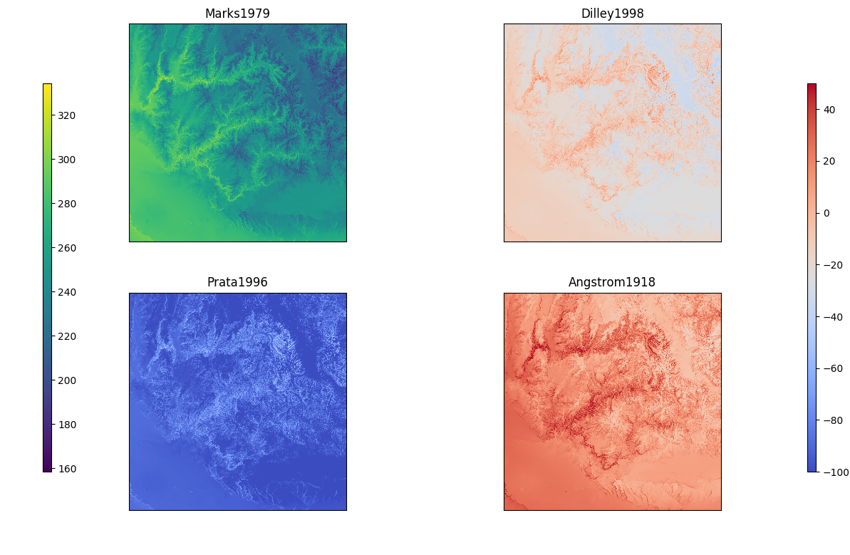
Fig. 5 The 4 different methods for estimating clear sky thermal radiation for a single time step. As compared to the Mark1979 method, the other methods provide a wide range in the estimated value of thermal radiation.

The topographic correct clear sky thermal radiation is further adjusted for cloud affects. Cloud correction is based on fraction of cloud cover, a cloud factor close to 1 meaning no clouds are present, there is little radiation added. When clouds are present, or a cloud factor close to 0, then additional long wave radiation is added to account for the cloud cover. Selecting one of the options below will change the equations used. The methods were chosen based on the study by Flerchinger et al (2009) [11], where $c=1-cloud\_factor$ .

Garen2005

Cloud correction is based on the relationship in Garen and Marks (2005) [17] between the cloud factor and measured long wave radiation using measurement stations in the Boise River Basin.

$L_{cloud} = L_{clear} * (1.485 - 0.488 * cloud\_factor)$

Unsworth1975

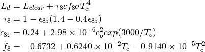
$L_d &= L_{clear} + \tau_8 c f_8 \sigma T^{4}_{c} \tau_8 &= 1 - \epsilon_{8z} (1.4 - 0.4 \epsilon_{8z}) \epsilon_{8z} &= 0.24 + 2.98 \times 10^{-6} e^2_o exp(3000/T_o) f_8 &= -0.6732 + 0.6240 \times 10^{-2} T_c - 0.9140 \times 10^{-5} T^2_c$

References: Unsworth and Monteith (1975) [18]

Kimball1982

$L_d &= L_{clear} + \tau_8 c \sigma T^4_c$

where the original Kimball et al. (1982) [19] was for multiple cloud layers, which was simplified to one layer. $T_c$ is the cloud temperature and is assumed to be 11 K cooler than $T_a$ .

References: Kimball et al. (1982) [19]

Crawford1999

$\epsilon_a = (1 - cloud\_factor) + cloud\_factor * \epsilon_{clear}$

References: Crawford and Duchon (1999) [20] where $cloud\_factor$ is the ratio of measured solar radiation to the clear sky irradiance.

The results from Flerchinger et al (2009) [11] showed that the Kimball1982 cloud correction with Dilley1998 clear sky algorthim had the lowest RMSD. The Crawford1999 worked best when combined with Angstrom1918, Dilley1998, or Prata1996.

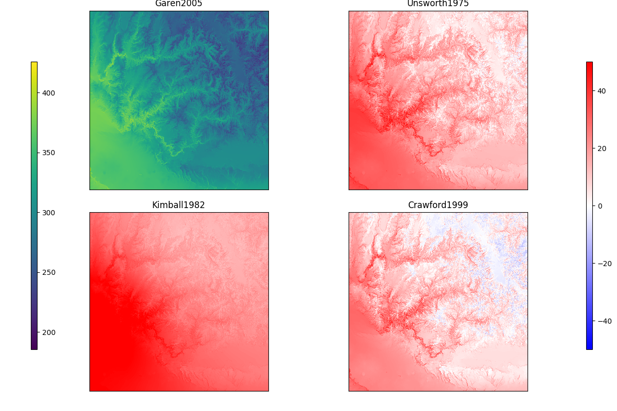
Comparing the 4 thermal cloud correction methods.

Fig. 6 The 4 different methods for correcting clear sky thermal radiation for cloud affects at a single time step. As compared to the Garen2005 method, the other methods are typically higher where clouds are present (i.e. the lower left) where the cloud factor is around 0.4.

The thermal radiation is further adjusted for canopy cover after the work of Link and Marks (1999) [10]. The correction is based on the vegetation’s transmissivity, with the canopy temperature assumed to be the air temperature for vegetation greater than 2 meters. The thermal radiation is adjusted by

$L_{canopy} = \tau_d * L_{cloud} + (1 - \tau_d) \epsilon \sigma T_a^4$

where $\tau_d$ is the optical transmissivity, $L_{cloud}$ is the cloud corrected thermal radiation, $\epsilon$ is the emissivity of the canopy (0.96), $\sigma$ is the Stephan-Boltzmann constant, and $T_a$ is the distributed air temperature.

Parameters:	thermalConfig – The [thermal] section of the configuration file

config¶: configuration from [thermal] section

thermal¶: numpy array of the precipitation

min¶: minimum value of thermal is -600 W/m^2

max¶: maximum value of thermal is 600 W/m^2

stations¶: stations to be used in alphabetical order

output_variables¶: Dictionary of the variables held within class smrf.distribute.thermal.ta that specifies the units and long_name for creating the NetCDF output file.

variable¶: ‘thermal’

dem¶: numpy array for the DEM, from smrf.data.loadTopo.topo.dem

veg_type¶: numpy array for the veg type, from smrf.data.loadTopo.topo.veg_type

veg_height¶: numpy array for the veg height, from smrf.data.loadTopo.topo.veg_height

veg_k¶: numpy array for the veg K, from smrf.data.loadTopo.topo.veg_k

veg_tau¶: numpy array for the veg transmissivity, from smrf.data.loadTopo.topo.veg_tau

sky_view¶: numpy array for the sky view factor, from smrf.data.loadTopo.topo.sky_view

distribute(date_time, air_temp, vapor_pressure=None, dew_point=None, cloud_factor=None)[source]¶

Distribute for a single time step.

The following steps are taken when distributing thermal:

Calculate the clear sky thermal radiation from

smrf.envphys.core.envphys_c.ctopotherm
Correct the clear sky thermal for the distributed cloud factor
Correct for canopy affects

Parameters:	date_time – datetime object for the current step air_temp – distributed air temperature for the time step vapor_pressure – distributed vapor pressure for the time step dew_point – distributed dew point for the time step cloud_factor – distributed cloud factor for the time step measured/modeled

distribute_thermal(data, air_temp)[source]¶

Distribute given a Panda’s dataframe for a single time step. Calls smrf.distribute.image_data.image_data._distribute. Used when thermal is given (i.e. gridded datasets from WRF). Follows these steps:

Distribute the thermal radiation from point values
Correct for vegetation

Parameters:	data – thermal values air_temp – distributed air temperature values

distribute_thermal_thread(queue, data)[source]¶

Distribute the data using threading and queue. All data is provided and distribute_thread will go through each time step and call smrf.distribute.thermal.th.distribute_thermal then puts the distributed data into the queue for thermal. Used when thermal is given (i.e. gridded datasets from WRF).

Parameters:	queue – queue dictionary for all variables data – pandas dataframe for all data, indexed by date time

distribute_thread(queue, date)[source]¶

Distribute the data using threading and queue. All data is provided and distribute_thread will go through each time step and call smrf.distribute.thermal.th.distribute then puts the distributed data into the queue for thermal.

Parameters:	queue – queue dictionary for all variables data – pandas dataframe for all data, indexed by date time

initialize(topo, data)[source]¶

Initialize the distribution, calls smrf.distribute.image_data.image_data._initialize for gridded distirbution. Sets the following from smrf.data.loadTopo.topo

veg_height
veg_tau
veg_k
sky_view
dem

Parameters:	topo – `smrf.data.loadTopo.topo` instance contain topographic data and infomation data – data Pandas dataframe containing the station data, from `smrf.data.loadData` or `smrf.data.loadGrid`

smrf.distribute.vapor_pressure module¶

class smrf.distribute.vapor_pressure.vp(vpConfig, precip_temp_method)[source]¶

Bases: smrf.distribute.image_data.image_data

The vp class allows for variable specific distributions that go beyond the base class

Vapor pressure is provided as an argument and is calcualted from coincident air temperature and relative humidity measurements using utilities such as IPW’s rh2vp. The vapor pressure is distributed instead of the relative humidity as it is an absolute measurement of the vapor within the atmosphere and will follow elevational trends (typically negative). Were as relative humidity is a relative measurement which varies in complex ways over the topography. From the distributed vapor pressure, the dew point is calculated for use by other distribution methods. The dew point temperature is further corrected to ensure that it does not exceed the distributed air temperature.

Parameters:	vpConfig – The [vapor_pressure] section of the configuration file

config¶: configuration from [vapor_pressure] section

vapor_pressure¶: numpy matrix of the vapor pressure

dew_point¶: numpy matrix of the dew point, calculated from vapor_pressure and corrected for dew_point greater than air_temp

min¶: minimum value of vapor pressure is 10 Pa

max¶: maximum value of vapor pressure is 7500 Pa

stations¶: stations to be used in alphabetical order

output_variables¶: Dictionary of the variables held within class smrf.distribute.vapor_pressure.vp that specifies the units and long_name for creating the NetCDF output file.

variable¶: ‘vapor_pressure’

distribute(data, ta)[source]¶

Distribute air temperature given a Panda’s dataframe for a single time step. Calls smrf.distribute.image_data.image_data._distribute.

The following steps are performed when distributing vapor pressure:

Distribute the point vapor pressure measurements
Calculate dew point temperature using

smrf.envphys.core.envphys_c.cdewpt
Adjust dew point values to not exceed the air temperature

Parameters:	data – Pandas dataframe for a single time step from precip ta – air temperature numpy array that will be used for calculating dew point temperature

distribute_thread(queue, data)[source]¶

Distribute the data using threading and queue. All data is provided and distribute_thread will go through each time step and call smrf.distribute.vapor_pressure.vp.distribute then puts the distributed data into the queue for:

vapor_pressure
dew_point

Parameters:	queue – queue dictionary for all variables data – pandas dataframe for all data, indexed by date time

initialize(topo, data)[source]¶

Initialize the distribution, calls smrf.distribute.image_data.image_data._initialize. Preallocates the following class attributes to zeros:

Parameters:	topo – `smrf.data.loadTopo.topo` instance contain topographic data and infomation data – data Pandas dataframe containing the station data, from `smrf.data.loadData` or `smrf.data.loadGrid`

smrf.distribute.wind module¶

class smrf.distribute.wind.wind(windConfig, distribute_drifts, wholeConfig, tempDir=None)[source]¶

Bases: smrf.distribute.image_data.image_data

The wind class allows for variable specific distributions that go beyond the base class.

Estimating wind speed and direction is complex terrain can be difficult due to the interaction of the local topography with the wind. The methods described here follow the work developed by Winstral and Marks (2002) and Winstral et al. (2009) [21] [22] which parameterizes the terrain based on the upwind direction. The underlying method calulates the maximum upwind slope (maxus) within a search distance to determine if a cell is sheltered or exposed. See smrf.utils.wind.model for a more in depth description. A maxus file (library) is used to load the upwind direction and maxus values over the dem. The following steps are performed when estimating the wind speed:

Adjust measured wind speeds at the stations and determine the wind

direction componenets
Distribute the flat wind speed
Distribute the wind direction components
Simulate the wind speeds based on the distribute flat wind, wind

direction, and maxus values

After the maxus is calculated for multiple wind directions over the entire DEM, the measured wind speed and direction can be distirbuted. The first step is to adjust the measured wind speeds to estimate the wind speed if the site were on a flat surface. The adjustment uses the maxus value at the station location and an enhancement factor for the site based on the sheltering of that site to wind. A special consideration is performed when the station is on a peak, as artificially high wind speeds can be calcualted. Therefore, if the station is on a peak, the minimum maxus value is choosen for all wind directions. The wind direction is also broken up into the u,v componenets.

Next the flat wind speed, u wind direction component, and v wind direction compoenent are distributed using the underlying distribution methods. With the distributed flat wind speed and wind direction, the simulated wind speeds can be estimated. The distributed wind direction is binned into the upwind directions in the maxus library. This determines which maxus value to use for each pixel in the DEM. Each cell’s maxus value is further enhanced for vegetation, with larger, more dense vegetation increasing the maxus value (more sheltering) and bare ground not enhancing the maxus value (exposed). With the adjusted maxus values, wind speed is estimated using the relationships in Winstral and Marks (2002) and Winstral et al. (2009) [21] [22] based on the distributed flat wind speed and each cell’s maxus value.

When gridded data is provided, the methods outlined above are not performed due to the unknown complexity of parameterizing the gridded dataset for using the maxus methods. Therefore, the wind speed and direction are distributed using the underlying distribution methods.

Parameters:	windConfig – The [wind] section of the configuration file

config¶: configuration from [vapor_pressure] section

wind_speed¶: numpy matrix of the wind speed

wind_direction¶: numpy matrix of the wind direction

veg_type¶: numpy array for the veg type, from smrf.data.loadTopo.topo.veg_type

_maxus_file¶: the location of the maxus NetCDF file

maxus¶: the loaded library values from _maxus_file

maxus_direction¶: the directions associated with the maxus values

min¶: minimum value of wind is 0.447

max¶: maximum value of wind is 35

stations¶: stations to be used in alphabetical order

output_variables¶: Dictionary of the variables held within class smrf.distribute.wind.wind that specifies the units and long_name for creating the NetCDF output file.

variable¶: ‘wind’

convert_wind_ninja(t)[source]¶

Convert the WindNinja ascii grids back to the SMRF grids and into the SMRF data streamself.

Parameters:	t – datetime of timestep
Returns:	wind speed numpy array wd: wind direction numpy array
Return type:	ws

distribute(data_speed, data_direction, t)[source]¶

Distribute given a Panda’s dataframe for a single time step. Calls smrf.distribute.image_data.image_data._distribute.

Follows the following steps for station measurements:

Adjust measured wind speeds at the stations and determine the wind

direction componenets
Distribute the flat wind speed
Distribute the wind direction components
Simulate the wind speeds based on the distribute flat wind, wind

direction, and maxus values

Gridded interpolation distributes the given wind speed and direction.

Parameters:	data_speed – Pandas dataframe for single time step from wind_speed data_direction – Pandas dataframe for single time step from wind_direction t – time stamp

distribute_thread(queue, data_speed, data_direction)[source]¶

Distribute the data using threading and queue. All data is provided and distribute_thread will go through each time step and call smrf.distribute.wind.wind.distribute then puts the distributed data into the queue for wind_speed.

Parameters:	queue – queue dictionary for all variables data – pandas dataframe for all data, indexed by date time

initialize(topo, data)[source]¶

Initialize the distribution, calls smrf.distribute.image_data.image_data._initialize. Checks for the enhancement factors for the stations and vegetation.

Parameters:	topo – `smrf.data.loadTopo.topo` instance contain topographic data and infomation data – data Pandas dataframe containing the station data, from `smrf.data.loadData` or `smrf.data.loadGrid`

simulateWind(data_speed)[source]¶

Calculate the simulated wind speed at each cell from flatwind and the distributed directions. Each cell’s maxus value is pulled from the maxus library based on the distributed wind direction. The cell’s maxus is further adjusted based on the vegetation type and the factors provided in the [wind] section of the configuration file.

Parameters:	data_speed – Pandas dataframe for a single time step of wind speed to make the pixel locations same as the measured values

stationMaxus(data_speed, data_direction)[source]¶

Determine the maxus value at the station given the wind direction. Can specify the enhancemet for each station or use the default, along with whether or not the station is on a peak which will ensure that the station cannot be sheltered. The station enhancement and peak stations are specified in the [wind] section of the configuration file. Calculates the following for each station:

flatwind
u_direction
v_direction

Parameters:	data_speed – wind_speed data frame for single time step data_direction – wind_direction data frame for single time step